|
|||||||||||||||||||||||||||||||||||||||||||||||||||||||||||||||||||||||||||||||||||||||||||||||||||||
|
|
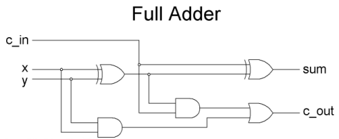
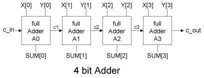
VeriLogger Tutorial A: Basic Verilog SimulationThis tutorial demonstrates the basic simulation features of VeriLogger Pro. It teaches you how to create and manage a project and how to build, simulate, and debug your design. It also demonstrates the graphical test bench generation features that are unique to VeriLogger Pro. This is a stand alone tutorial which you should be able to complete without reading any of the other tutorials. However, if you plan to make extensive use of the graphical stimulus generation features then you may also want to perform the Basic Drawing and Timing Analysis tutorial and Waveform Generation and Bus tutorial which cover the time-saving features of the timing diagram editor. In this tutorial, you will compile and simulate a 4-bit adder and a test bench module contained in files add4.v and add4test.v. Figure 1 shows a schematic of the circuit. Later in the tutorial you learn to graphically enter the stimulus vectors instead of using a test bench module. Also you will get to practice using the basic debugging features of breakpoints, single stepping, and viewing different signals in the file.
Figure 1: Schematic of the 4-bit adder simulated in this tutorial. Part 1: Project Management and SimulationIn this section, you will create, build, and simulate a project. VeriLogger uses a project to control all aspects of simulation and design including specifying the files to be simulated, controlling simulation options, and setting watches on signals. The project also stores the hierarchical structure of the Verilog components contained in the design and displays this information on the tree control in the Project window. 1.1 Add Files to the Project The first step in creating a project is to add Verilog files to the project tree window and save the project. To add a file to the project:
1.2 Build the Tree and use the Editor Windows In this section we will build the project tree and use the Editor windows to view the source code. When files are first added to the project, you can see the file name but you cannot see a hierarchical view of the modules inside the files. To view the internal modules on the project tree you must first build or run a simulation. The build command compiles the Verilog files and builds the Verilog tree. It does not run a simulation. For large projects build lets you quickly construct the tree without having to wait for a simulation to run. To build a project:
All sub-modules can be viewed by descending the top-level module's tree. When the tree is expanded it can display the signals, ports, and components contained in each module. Expand the tree by using the + buttons or by using the node context menu Expand Item. Try both methods for expanding the tree:
Double clicking on a particular module or node in the Project Tree causes an editor to open and display the relevant source code. Let's view some source code:
The editors can be used to edit and write Verilog source code. Most of the Editor window functions are accessed from the Editor menu tree.
Chapter 4: Editor Functions in the on-line VeriLogger help manual has more information on using the Editor windows. 1.3 Simulate the Project When we built the project in the last section, the names of the internal signals in the top-level module were automatically added to the Diagram window. This feature allows you to quickly set up a project and start simulating and debugging without having to stop and specify a set of signals. For large projects you may want to turn off this feature by choosing the Project > Project Settings menu and un-checking the Grab top level signals check box. For small projects the automatic signal watches save a lot of time so we will leave it on for the tutorial. First, let's simulate with the default signals:
1.4 Watch and View Internal Signals With VeriLogger you can watch any combination of signals listed under the top-level module tree. To demonstrate this we will set watches on the sum outputs for the full adders sub-modules that make up the 4-bit adder:
To remove signals from the watch list, delete them from the Diagram window:
Next we will experiment with different ways to view waveforms in the Diagram window:
1.5 Save the Project, Waveforms and Source Code Next we will learn to save the project, waveforms, and source code. The project saves the simulation options and the names of the files contained on the project tree. It does not save the source code or the watched signals. To save the project:
The watched signals are saved using timing diagram files. By making the watched signals separate from the project file, VeriLogger lets you set up different sets of watched signals so that you do not have to watch your entire design each time you simulate. Also watching small sections of your design makes it easier to detect bugs in a particular section and speeds up simulation execution. In the evaluation version of VeriLogger you cannot save the waveforms, however in the full version you can save using the following menu command:
Each time you simulate, every open editor is queried to determine if the source code needs to be saved before the simulation starts. If you need to save the code before you are ready to perform a simulation, use one of the following menu options:
To re-open a VeriLogger Project, first open the project and then load the timing diagram files. 1.6 Configure the Project for Part 2 Now we will set up the project for the next section by removing the test bench file and saving the project under a different name. To remove add4test.v from the project:
Part 2: Graphical Test Bench GenerationIn this section you will draw and simulate a test bench using the timing diagram editor. 2.1 Build the Project and Examine the Black Signals In the previous section, all the signals were purple to indicate that they were simulated signals that were generated by the Verilog code. In this section we have deleted the testbed module and the new top level module has input port signals that are not being driven by any other module in the project. To verify this:
2.2 Use the Debug Run Simulation Mode VeriLogger has two simulation modes: Auto Run and Debug Run. The simulation mode is displayed on the left most button on the simulation button bar. In the Debug Run mode, simulations are started only when the user presses the Run or Single Step buttons (similar to a standard Verilog simulator). In Auto Run mode the simulator will automatically run a simulation each time a waveform is edited in the Waveform window. This mode makes it easy to quickly test small modules and perform bottom-up testing. While drawing the original test bench we will set the simulator to Debug Run mode:
2.3 How to Draw Waveforms If you are already familiar with SynaptiCAD's timing diagram editing environment, skip ahead to Section 2.5 where you will draw stimulus vectors and use the Virtual State edit box to define the values for the x and y busses. If this is your first time using a SynaptiCAD timing diagram editor then we will first draw several random waveforms to familiarize you with the drawing environment.
Your drawing should be a mess, or at least look nothing like Figure 2 located in Section 2.5. 2.4 How to Edit Waveforms There are four main editing techniques used to modify existing signals (Note: these techniques will not work on clocks and simulated signals). The most commonly used technique is the dragging of signal transitions to adjust their location. The other three techniques all act on signal segments (the waveforms between two consecutive signal transitions). The segment waveform can be changed, deleted, or a new segment can be inserted within another segment. Use each of the following techniques:
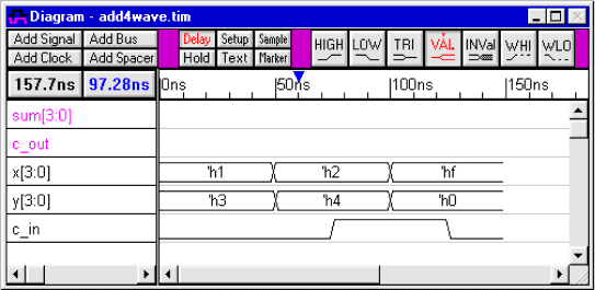
For more detailed instructions, read the TestBencher and WaveFormer on-line help Chapter 1: Signals and Waveforms. 2.5 Draw the Stimulus Waveforms Now use the above techniques to edit the signals so they have roughly the same transitions and graphical states as the signals in the figure below. This is not the normal way to create a timing diagram, but it will teach you how to use the editing features of SynaptiCAD's timing diagram editor. Make sure you try all the editing techniques.
Figure 2: Stimulus vectors for the 4-bit adder circuit Next, edit the virtual bus states of the valid segments on the x and y buses:
At this point, the c_in, x[3:0], and y[3:0] signals should look like Figure 2. Exact placement of edges is not required for this tutorial. 2.6 Simulate using the Auto Run Simulation Mode Currently the simulator is in Debug Run mode, so simulations are started only when the Run button is pressed. Start a simulation:
Next we will demonstrate the Auto Run mode which allows interactive debugging of modules. This mode is especially useful for debugging small modules.
2.7 Import and Generate Waveforms The most difficult and tedious part of designing test benches is accurately entering the waveform data. VeriLogger accelerates this process by accepting waveform data via six different methods: Verilog code, drawing, spreadsheets, simulator output, HP logic analyzer capture, and equation generation. So far we have demonstrated the drawing of waveforms and the use of standard Verilog code which are excellent choices for designing small test benches. However, for large test benches it is easier to use automated techniques to generate your data. The TestBencher and WaveFormer on-line help Chapter 13: Stimulus Generation and Waveform Import covers the spreadsheet, simulator import, and HP Logic analyzer features. The equation-based generation of waveforms is covered in Chapter 11: Waveform Equation Generation. Let us quickly demonstrate the waveform equation features using the following steps:
You can also automatically label waveforms by using the Label Waveform Equation functions. These are more complex than the waveform equations so you will have to read Chapter 11 in the TestBencher and WaveFormer manual to get the full benefit of these features.
Part 3: Breakpoints, Stepping, and TracingIf you would like to practice debugging, first read the Getting Started and Chapter 3: Simulation and Debug Functions chapters in the on-line VeriLogger Help. Next, introduce a syntax error into the add4.v file and attempt to find it using the Errors tag in the Report window. Fix the syntax error. Then introduce a semantic error in the full adder code so that it does not handle the carry correctly. Use breakpoints and single-step debugging to locate the error. |
 on the simulation button bar.
 to expand the project tree. Notice that the sub-nodes of Signals and Components are not expanded.
 on the simulation button bar. This causes a simulation to start and run until the end of the simulation
time or until a breakpoint is reached. The Diagram window should contain purple waveforms.
on the simulation button bar. This causes a simulation to start and run until the end of the simulation
time or until a breakpoint is reached. The Diagram window should contain purple waveforms.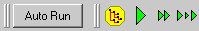
|
|